AoC2021 Day22: Reactor Reboot

December 2021

The Problem

Advent of Code 2021 – Day 22 . After 21 days of rough submarine life on the quest to find the misplaced sleigh keys somewhere deep in the ocean, it turns out the extreme depths have overloaded the submarine’s reactor and it needs to be rebooted.

The submarine reactor exists in the form of a 3d-grid that can be entirely filled with unit cubes (cubes whose edges have unit length). Each unit cube undergoes a series of switch-on-or-off instructions. After all instructions have been executed for all unit cubes, the final state of the grid constitutes the rebooted reactor. In this article I’ll be going over my solution to this puzzle and some key procedures required to implement it. My solution is based on splitting cuboids¹.

Part 1 – Reactor Initialization

As explained in the documentation:

The reactor core is made up of a large 3-dimensional grid made up entirely of cubes, one cube per integer 3-dimensional coordinate (x,y,z). Each cube can be either on or off; at the start of the reboot process, they are all off.

To reboot the reactor, you just need to set all of the cubes to either on or off by following a list of reboot steps (your puzzle input). Each step specifies a cuboid (the set of all cubes that have coordinates which fall within ranges for x, y, and z) and whether to turn all of the cubes in that cuboid on or off.

The initialization procedure only uses cubes that have x, y, and z positions of at least -50 and at most 50². For now, ignore cubes outside this region.

Q: Execute the reboot steps. How many cubes are on?

This is the first example input:

on x=10..12,y=10..12,z=10..12
on x=11..13,y=11..13,z=11..13
off x=9..11,y=9..11,z=9..11
on x=10..10,y=10..10,z=10..10

By now we know that we’re operating with a 3d-grid fillable with unit cubes (simply cubes going forward). Then, some complexity is added: in the instructions cubes are only referenced indirectly, since each instruction line actually describes a cuboid —which by extension contains all cubes inside it. In simple terms a cuboid is a 3d rectangle, aka a rectangular prism.

Consider the first line of the example above, on x=10..12,y=10..12,z=10..12, it’s a switch-on instruction followed by start-to-end ranges of the sides of a cuboid—in fact a 3x3x3 cuboid filled with 27 cubes. Each of these cubes is given by a 3d coord: (10,10,10), (10,10,11), (10,10,12), ..., (12,12,12). The actual puzzle input consists of 420 such formatted instructions.

Polygons & Voxels

This is a good point to stop and think about coordinates for a bit. Typically, we understand coordinates as sets of N numbers that exactly locate a point in dimension N; thus a single 3d point is given by the 3d coordinate (x, y, z). Each coordinate represents a vertex; connections between vertices create edges; and three or more connected edges become a polygon (the triangle is the simplest polygon, followed by the quadrilateral, and so on)³.

Under this coordinate format, storing a single cube would require storing eight 3d coordinates, one for each of its vertices (and vertex ordering would have to be meaningful as well, to indicate the connection sequence to actually create the cube). For the 27 cubes of the first entry line that would mean 8x27 = 216 coordinate points, that would be highly inefficient, especially considering how the cubes are stacked on top of each other seamlessly, forming a bounding volume (filled with empty space).

This exercise utilizes voxels instead:

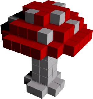
A voxel represents a single sample, or data point, on a regularly spaced, three-dimensional grid. This data point can consist of a single piece of data, such as an opacity, or multiple pieces of data, such as a color in addition to opacity. A voxel represents only a single point on this grid, not a volume; the space between each voxel is not represented in a voxel-based dataset.

Figure 1. A Voxel Shroom

Voxels help with compression, though we still need to be wary of off-by-one errors ; in particular notice that for any dimensional range both ends of the interval should be included. With the notion of voxel under our belts we move on to implement the solution for Part 1⁴.

Parsing the Input

def integers(text, negative=True):
    """Extract integers from text."""
    return mapt(int, re.findall(r"-?\d+" if negative else r"\d+", text))

steps = [(row.split(" ")[0], integers(row)) for row in data]
# [
#   ('on', (10, 12, 10, 12, 10, 12)),
#   ('on', (11, 13, 11, 13, 11, 13)),
#   ('off', (9, 11, 9, 11, 9, 11)),
#   ('on', (10, 10, 10, 10, 10, 10)),
# ]

Initialization Code

The implementation for Part 1 is fairly straightforward. As discussed above, we iterate through every reboot step, extract the cuboid, calculate and truncate its dimensional ranges (adding +1 to end-ranges in lines 8, 9 and 10 to make them inclusive), and then we use these ranges as a bounding volume to extract every single cube inside. Next, depending on the switching command (on/off), we add or remove these cubes to/from the tracking set. The number of elements in the set at the end is the answer: 527915.

 1def initialize_reactor(steps):
 2    """--- Day 22: Reactor Reboot ---"""
 3    cubes = set()
 4    for switch, step in steps:
 5        x1, x2, y1, y2, z1, z2 = step
 6        new_cuboid = {  # inclusive range. truncate from -50 to 50
 7            (x, y, z)
 8            for x in range(max(x1, -50), min(x2, 50) + 1)
 9            for y in range(max(y1, -50), min(y2, 50) + 1)
10            for z in range(max(z1, -50), min(z2, 50) + 1)
11        }
12        if switch == "on":
13            cubes |= new_cuboid  # set union
14        else:
15            cubes -= new_cuboid  # set removal
16    return len(cubes)

Part 2 – Reactor Reboot

Now that the initialization procedure is complete, you can reboot the reactor. Starting with all cubes off, run all of the reboot steps for all cubes in the reactor.

As suspected in Part 1 the size constraint limiting voxels to -50 and 50 has been dropped, and now we have a new problem in our hands, let’s see why. In Part 1 the size constraint limits the maximum volume of the reactor to holding 101x101x101 = 1'030'301 cubes, or roughly one million. Each cube takes up 48 bytes in memory, requiring at most 48*10**6/1024**2 ~ 45 MB in total. For reference, the solution to Part 1 ended up using 527'915 or ~51% of reactor volume capacity.

Quick inspection of the actual input reveals that lifting this constraint has huge implications. Namely, it causes the maximum length each dimension is allowed to span to shoot up by a factor of ~2000x. That means now the reactor can hold up to ~7.4 quadrillion cubes (i.e., 15 zeros), and if we were to keep them all in memory we would require 316 PB. Oof, things escalated quickly. The problem of course, is that we are cutting up each cuboid into all its constituent cubes—an unnecessary level of granularity. We’ll have to devise a more efficient solution.

# back-of-the-envelope dimensionality calculations for part 2
x_min, x_max = min([s[0] for _, s in steps]), max([s[1] for _, s in steps])
y_min, y_max = min([s[2] for _, s in steps]), max([s[3] for _, s in steps])
z_min, z_max = min([s[4] for _, s in steps]), max([s[5] for _, s in steps])
print(f"x: {(x_min, x_max)}, y: {(y_min, y_max)}, z: {(z_min , z_max)}")
# x: (-96513, 97051), y: (-99029, 95078), z: (-98435, 98668)
x_sz = x_max - x_min + 1
y_sz = y_max - y_min + 1
z_sz = z_max - z_min + 1
print(f"x_len: {x_sz}, y_len: {y_sz}, z_len: {z_sz}")
# x_len: 193565, y_len: 194108, z_len: 197104
print(f"max vol: {round((x_sz * y_sz * z_sz)/ 10 ** 15, 1)}")
# ~7.4 Quadrillion
print(round(48 * (x_sz * y_sz * z_sz) / 1024 ** 5, 1))
# ~316 PB

The Inclusion–Exclusion Principle

Consider the second step in the initial example, on x=11..13,y=11..13,z=11..13. Once again this is a cuboid with a switch-on instruction and with 27 cubes inside. Note though, of these 27 cubes, 8 have already been turned on by the previous step (i.e., these 8 cubes make up the intersection region), thus the second cuboid only turns on its remaining, non-intersected 19 cubes—for a total of 46 on cubes.

In general, every time we join two cuboids, there is the possibility of an overlap, and if we don’t remove the overlapping region from the total, then we incur double counting. In short, via the inclusion-exclusion principle , we want to enforce the following:

\[ |A \cup B| = |A| + |B| - |A \cap B| \hspace{1cm} (1)\]

Equation (1) is the starting point for a more systematic way to account for intersections.

Splitting Cuboids

The key observation here is that after removing the intersection of A and B from A—assuming the intersection is not empty—then A becomes a new, smaller figure. In fact the new figure is not a cuboid anymore, since it is missing a chunk of voxels, nonetheless it can still be split into a collection of smaller cuboids (minikuboids).

This result is amazingly convenient because now instead of having to track \(n\) minikuboids (19 in our ongoing example), it is enough to track at most 6, and at least 3, depending on the nature of the intersection.

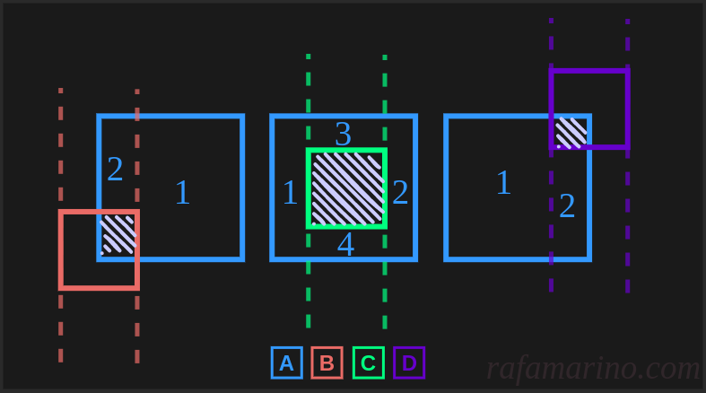
Figure 2 illustrates the intuition behind this idea in 2d, by showing how rectangle A intersects with three other rectangles (B, C and D). After determining the intersection region, we cut A vertically at the other rectangle’s start-and-end points, resulting in mini-rectangle splits. Depending on the geometry of each case, A may be split in two, three or four mini-rectangles. Two-dimensional split mechanics extend over to cuboids by adding a few book-keeping adjustments for the \(z\) axis.

Figure 2. Splitting Rectangles

Pseudocode Strategy

The inclusion-exclusion principle and the cuboid-splitting procedure are key components of the new design. The pseudocode block below outlines the strategy:

 1def REBOOT_REACTOR(reboot_steps):
 2    """Reboot reactor"""
 3    reactor = []
 4    for step in reboot_steps:
 5        temp = []
 6        for cuboid in reactor:
 7            minikuboids = cuboid.subtract(step.cuboid)
 8            temp.append(minikuboids)
 9        reactor = temp
10        if step.switch is on:
11            reactor.append(step.cuboid)
12    return sum(cuboid.volume() for cuboid in reactor)

We start with an empty reactor list, then we execute each instruction in reboot_steps sequentially—and for each instruction we create a placeholder, temp. Next, we iterate over every cuboid in the current reactor, and for each cuboid we subtract from it its intersection with the current instruction’s cuboid, step.cuboid.

This subtraction procedure will split the cuboid into minikuboids, which are then added to temp; the latter in turn becomes the new reactor at the end of the loop. We’re not yet finished as we still need to check whether the current instruction is a case of “on” or “off”. In the “on” case, add step.cuboid to the reactor (you can safely ignore it otherwise: in the “off” case it will have already been removed after the subtraction loop ends). In the end, after all instructions are processed, the volume of the reactor is exactly the sum of the volumes of its cuboids.

The Cuboid Dataclass

It’s time to code it. Following from the previous section, we need to support the computation of cuboid volume, intersection and subtraction. For this I will implement a Cuboid dataclass . Dataclass is a strong Python module that reduces class-creation boilerplate and provides convenient functionality and notation for immutable objects, among other things. The Cuboid class should have start and end attributes for each of the three dimensions x, y, z. As well as methods for each of the operations mentioned above.

Note once more that voxel ranges are inclusive, so we need to add a +1 to length calculations just like before, this can be done outside or inside the class. I’ve found the math in the former case to be a lot cleaner, therefore the Cuboid class will be designed to expect end ranges with a +1 adjustment at instantiation time, like so:

Cuboid(x1, x2+1, y1, y2+1, z1, z2+1)

Let’s briefly discuss the three methods. For cuboids A and B:

• A.volume()—this is simply side \(x\) by side \(y\) by side \(z\) of A.
• A.intersects(B)—two cuboids intersect if they overlap in all three dimensions simultaneously. Each dimension can be checked separately but they all need to hold. Take \(x\), cuboids A and B overlap in \(x\) if and only if the start of A is less than or equal to the end of B and the end of A is greater than or equal to the start of B. Repeat for \(y\) and \(z\). But, because we extended the end ranges (+1), we drop the equality and make it strict. Return a boolean if all axes hold.
• A.subtract(B)—first we check if A and B intersect, if they don’t, then return A unchanged. Otherwise, extract the intersection and call it cuboid C. Using C, and following the inspiration from Figure 2, split A in six minikuboids and yield them.

See the implementation below.

 1@dataclass(frozen=True)
 2class Cuboid:
 3    x1: int
 4    x2: int
 5    y1: int
 6    y2: int
 7    z1: int
 8    z2: int
 9
10    def volume(self):
11        x_len = (self.x2 - self.x1)
12        y_len = (self.y2 - self.y1)
13        z_len = (self.z2 - self.z1)
14        return x_len * y_len * z_len
15
16    def intersects(a, b):
17        x_check = a.x1 < b.x2 and a.x2 > b.x1
18        y_check = a.y1 < b.y2 and a.y2 > b.y1
19        z_check = a.z1 < b.z2 and a.z2 > b.z1
20        return x_check and y_check and z_check
21
22    def subtract(a, b):
23        if not a.intersects(b):
24            yield a
25        else:
26            c = Cuboid(
27                min(max(b.x1, a.x1), a.x2),
28                min(max(b.x2, a.x1), a.x2),
29                min(max(b.y1, a.y1), a.y2),
30                min(max(b.y2, a.y1), a.y2),
31                min(max(b.z1, a.z1), a.z2),
32                min(max(b.z2, a.z1), a.z2),
33            )
34
35            yield Cuboid(a.x1, c.x1, a.y1, a.y2, a.z1, a.z2)
36            yield Cuboid(c.x2, a.x2, a.y1, a.y2, a.z1, a.z2)
37            yield Cuboid(c.x1, c.x2, a.y1, c.y1, a.z1, a.z2)
38            yield Cuboid(c.x1, c.x2, c.y2, a.y2, a.z1, a.z2)
39            yield Cuboid(c.x1, c.x2, c.y1, c.y2, a.z1, c.z1)
40            yield Cuboid(c.x1, c.x2, c.y1, c.y2, c.z2, a.z2)

The trickiest parts of the algorithm were definitely min-maxing the right boundaries to find the coordinates of the intersection cuboid C in the general case, and then using C to split A into six minikuboids. Cuboid.subtract() hides all this complexity away.

Note also that subtract() is functional by design: the same input will always map to the same output, which is either the calling cuboid or the same six minikuboids from the split—this is due to the immutability provided by dataclass' frozen=True. However, as alluded to in Figure 2, depending on the intersection case some of these minikuboids may be flat in one dimension, thus having zero volume and zero effect in the final tally.

Rebooting Code

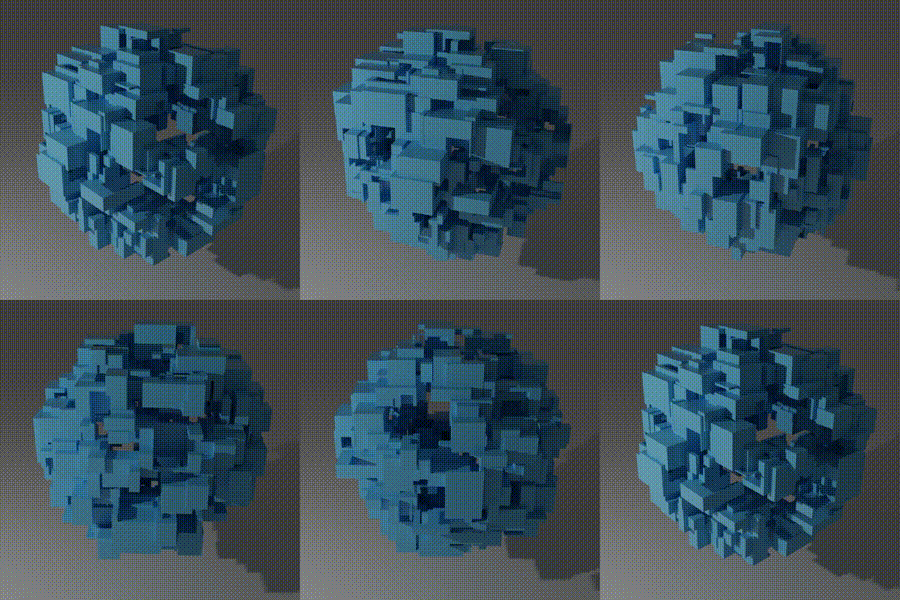
Finally, we run reboot_reactor which yields a total volume of 1218645427221987 (~16% of reactor volume capacity). There is a rendering of the final reactor at the top.

def reboot_reactor(reboot_steps):
    """--- Part Two ---"""
    reactor = []
    for switch, step in reboot_steps:
        x1, x2, y1, y2, z1, z2 = step
        new_cuboid = Cuboid(x1, x2 + 1, y1, y2 + 1, z1, z2 + 1)
        reactor_temp = []
        for cuboid in reactor:
            for minikuboid in cuboid.subtract(new_cuboid):
                reactor_temp.append(minikuboid)
        reactor = reactor_temp
        if switch == "on":
            reactor.append(new_cuboid)
    return sum(c.volume() for c in reactor)

(venv) $ python3 day22.py
# Part 2 -- On cubes after full reboot: 1218645427221987

Notes