Deeplearning.ai 01: Neural Networks

June 2020

Table of Contents

Summary

Notes for Andrew Ng’s Deep Learning Specialization Course 1.

Week 1

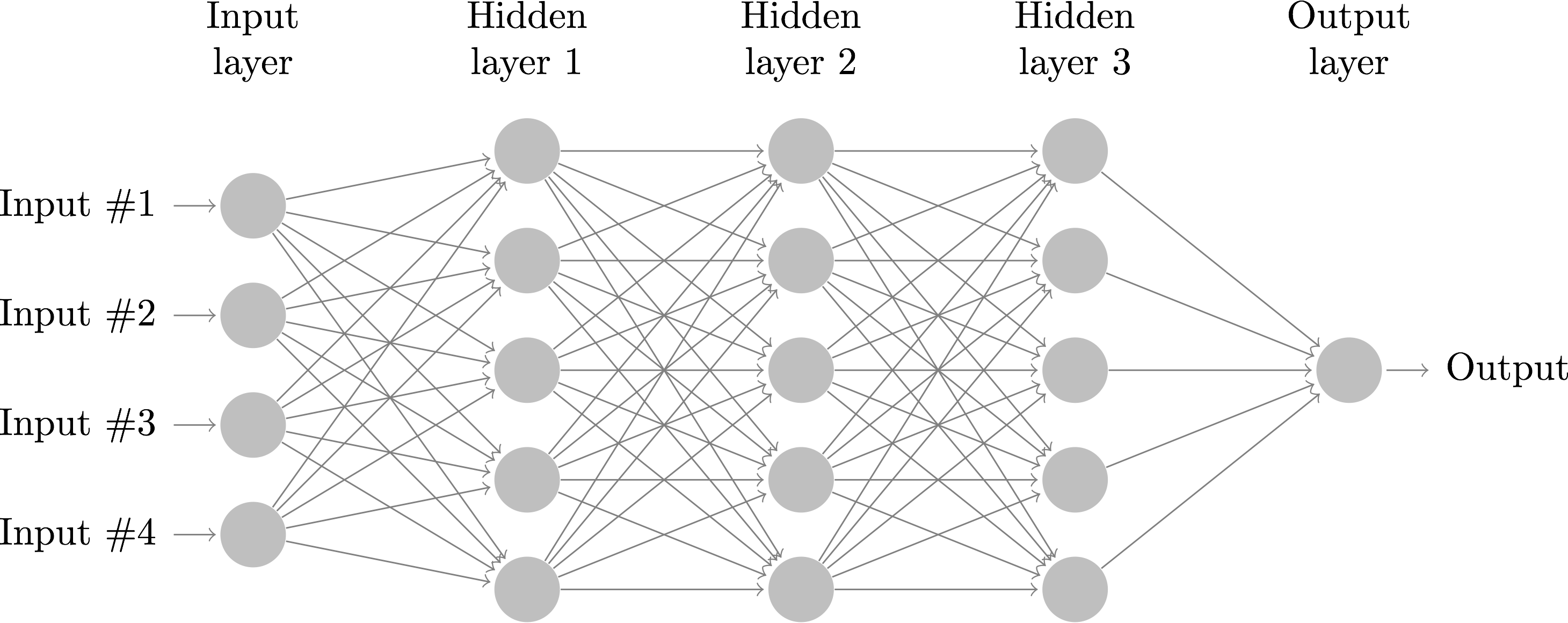
Representation of a Deep Neural Network:

A Deep Neural Network

Week 2

Image Representation

RGB channels: [Red, Green, Blue]
Example dimensions: 64x64x3. Unrolling RGB pixel intensity values results in a one-dimensional vector ∈ R (12288 x 1)

Notation:

m_train = training examples
m_test = test examples

Shapes for neural nets (NN):
$ Y = [y^1, y^2, … , y^m] \quad Y ∈ R(1 \times m) $

$ X = [x^1, x^2, … , x^m] \quad X ∈ R(n \times m) $

Y: a row vector. Each column contains the label for training example i
X: a matrix. Each column contains the feature vector for training example i

Linear Regression

\[ z = w^T.dot(x) + b\]

Where w is the vector of weights. There is one weight per feature. The prediction, ŷ, can be out of probability bounds [0, 1].

Vectors are conventionally initialized vertically. Therefore:

$ w^T $ is a row vector (ie horizontal)
$ x $ is a column vector (ie vertical)
$ w^T.dot(x) $ is a scalar and,
$ w^T.dot(x) + b $ is also a scalar

Logistic Regression (LR)

A probability is wanted:

$$ { ŷ = P(y=1 | x)} \quad ŷ \in [0,1] $$

The sigmoid function:

$$ \sigma(z) = \frac{1}{1+e^{-z}} = \frac{1}{1+ \frac{1}{e^z}} $$

if z is large: 1 / (1 + 0) ≈ 1
if z is small: 1 / (1 + BIG) ≈ 0

Activation function

$$ { \sigma(w^T.dot(X) + b) }$$

Goal: learn parameters W and b, so that ŷ^(i) is a good estimate for y^(i)
Note: superscript_i ^(i) refers to specific training-example_i

Next: in order to train a LR model, a loss/error function is needed

Example loss function

$$ { L(ŷ, y) = \frac{1}{2} (ŷ - y)^2 }$$

But, the squared error is not a good idea in logistic regression if it is to be trained with Gradient Descent (GD), because the optimization problem becomes non-convex, ie it has multiple local optima, GD may not ever converge on the global optimum. Instead, we can use (loss function for a single training example):

$$ { L(ŷ, y) = - ( ylogŷ + (1-y) log(1-ŷ) ) }$$

Intuition:

if y = 1: L(ŷ, y) = -logŷ (we want ŷ large)
if y = 0: L(ŷ, y) = -log(1-ŷ) (we want ŷ small)

The Cost Function extends the individual Loss Functions to the entire training set.

Generalization from Loss Function to Cost Function

To generalize the single-example Loss Function to a full training set with m examples, we do the following:

$$ { J(w, b) = (1/m) \sum_{i=1}^{m} L(ŷ^{(i)}, y^{(i)}) }$$

or, expanded out:

$$ { J(w, b) = -(1/m) \sum_{i=1}^{m} [ y^{(i)}logŷ^{(i)} + (1-y^{(i)}) log(1-ŷ^{(i)}) ] }$$

To train a Logistic Regression model, find parameters w, b (vectors, one element per feature) that minimize the Cost Function.

Gradient Descent

3Dimensions: [w, b, J(w,b)]
Goal: find values for w, b that minimize J(w, b)

Steps:

Initialize w and b: for LR almost any initialization method works, usually (0,0) but random initialization also works.
Take a step in the direction of the steepest descent
Stop algorithm when no longer minimizing

Basic Derivative Review:

slope == derivative == df(x)/x
“height/width” or “rise/run” or $ \Delta y/ \Delta x $
x nudged from 2.0 to 2.001, y goes from 6.0 to 6.003;
=> derivative = 3
Intuition dJ/dv: “if we were to take the value of v and change it a little, how would J change?"

Computation Graphs

Forward Propagation: Compute the output (left to right)
Backward Propagation: Compute derivatives (right to left)

Example function J(a,b,c):
u = bc; v = a + u; J = 3v
Chain rule:
dJ/da = dJ/dv * dv/da (a -> v -> J)

Convention for derivatives:

d(FinalOutputVariable)/d(variable) == dvar
Shortened to “dvar” (ie it is implied that the change of the intermediate variable “var” is assessed over the FinalOutputVariable)

Gradient Descent for Logistic Regression

Computation Graph:
[x1, w1, x2, w2, b] -> [Z = w1x1 + w2x2 + b] -> ŷ=a=sigmoid(Z) -> L(a,y)

Notation equivalence:
(L: loss function)
dw = dJ(w, b)/dw
db = dJ(w, b)/db
dZ = dL/dZ = dL(a,y)/dZ
da = dL/da = dL(a,y)/da
dw1 = dL/dw1
dw2 = dL/dw2

Derivative Calculus for LR:

(Y=ground truth vector doesn’t change, it makes no sense to compute dL/dy)
(X=feature vector, doesn’t change either)
da = -(y/a) + (1-y)/(1-a)
dZ = dL/da . da/dZ and,
da/dZ = a(1-a)
Therefore,
dZ = [-(y/a) + (1-y)/(1-a)] x a(1-a) = (a-y)
Then,
dw1 = x1dZ
dw2 = x2dZ
db = dZ

Gradient Descent on m examples

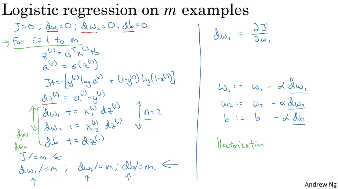
Once the entire loop is run (still one step), we can update the weights like so:

w1 := w1 - $\alpha$dw1
w2 := w2 - $\alpha$dw2
b := b - $\alpha$db

Vectorization – or the art of getting rid of explicit for loops in your code

Vectors are conventionally initialized vertically, therefore vec.T is horizontal

Computing usually slower by factor of 300x-400x using np.dot vs for loop

Parallelization instructions: Single instruction, multiple data (SIMD)

Vectorizing Logistic Regression

row-vector: a one-dimensional vector that grows horizontally, ie entries are in cols
col-vector: a one-dimensional vector that grows vertically, ie entries are in rows

X = [x^(1), x^(2), … , x^(m)] X ∈ R(n_x, m)(rows, cols)

ALERT: in traditional ML, x^(1), or the first column vector, is used to denote the feature vector containing values of feature x_1 for all training examples m. However, in deep learning, x^(1) denotes training example_1 across all its features. ie training examples grow horizontally and not vertically.

Prediction for training example 1

z^(1) = w^T.x^(1) + b
a^(1) = sigmoid(z^(1))

Predictions for 3 training examples

w^T.X + [b b b] (1,m) =
[w^T.x^(1)+b w^T.x^(2)+b w^T.x^(3)+b]
Z = [z^(1) z^(2) z^(3)] =

Z = np.dot(w^T, X) + b

(1 x 1; b is a scalar but Python broadcasts it)
A = [a^(1) a^(2) a^(3)]

Vectorizing Gradient Descent

dz^(i) = a^(i) - y^(i)
dZ = [dz^(1) dz^(2) dz^(3)]
Y = [y^(1) … y^(m)]
dZ = A - Y = [a^(1)-y^(1) a^(2)-y^(2) …]
(…)

Full Vectorization for GD (all training examples, one iteration)

Z = w^T.X + b = np.dot(w^T, X) + b
A = sigmoid(Z)
J =
dZ = A - Y
dw = (1/m) X dZ^T
db = (1/m) np.sum(dZ)

Updates:

w := w - $\alpha $dw
b := b - $\alpha $db

Broadcasting (ie auto-expand)

(axis=0) => across rows => vertically
(axis=1) => across cols => horizontal
(m,n) [+-*/] (1,n) ~> (m,n)
(m,n) [+-*/] (m,1) ~> (m,n)

Week 3

Review Computation Graph for Logistic Regression

[x, w, b] -> z = w^T.X + b -> a = sigmoid(z) -> L(a, y)

New notation for Neural Nets (NN)

2-layer NN: [Input layer -> (1) Hidden layer -> Output layer]
layer: (usually) vertical stack of nodes
superscript_1 = [1] = quantities associated with layer_1
$ a_j^{[i]}$ = activation unit j in layer i

Example Computation for 2-layer NN and 1 training example

W^[1] -> z^[1] = W^[1].x + b^[1] -> a^[1] = σ(z^[1]) -> z^[2] = W^[2].a^[1] + b^[2] -> a^[2] = σ(z^[2]) -> L(a^[2], y)

What happens inside each activation unit (ie. node)

Two steps of computation:

Step1: compute z = w^T.x + b
Step2: compute $\alpha(z)$ (ie activation)

Output Computation for Layer1_Node1 with 1 training example:
${ z_1^{[1]} = w_1^{[1]T}.dot(x^{(i)}) + b_1^{[1]}}$
${ a_1^{[1]}=\alpha(z_1^{[1]}) }$

NN Represetantion (1 training example)

Vectorizing across all m

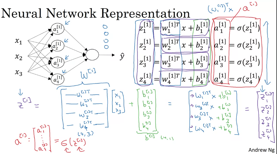
Associated parameters per layer:

$$ W^{layer}; b^{layer}; Z^{layer}; a^{layer} $$

Iterating through m examples (for loop version):
(Remember that each training example generates a prediction)

for i = 1 to m:
$ z^{[1][i]} = W^{[1]}.dot(x^{[i]}) + b^{[1]} $
$ a^{[1][i]}=\alpha(z^{[1][i]}) $
$ z^{[2][i]} = W^{[2]}.dot(a^{[1][i]}) + b^{[1]}$
$ a^{[2][i]}=\alpha(z^{[2][i]}) $

Extending to multiple training examples and vectorizing:

Vectorizing across all m

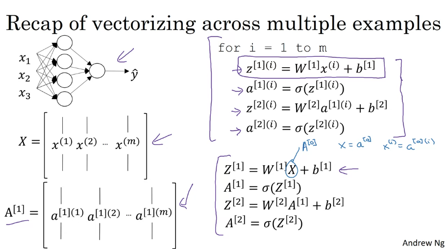
Activation matrix $ A^{[1]}$:

$ A^{[1]}$.axis=0 (rows): iterates through hidden units in layer1
$ A^{[1]}$.axis=1 (cols): iterates through training examples in layer1
Intuition: each hidden unit is “activated” iteratively by each training example

Activation functions

Activation functions are non-linear functions denoted by $g(Z^{[i]})$, where i represents the layer. Different layers can use different activation functions. Some common activation functions are:

Why does a NN need a non-linear activation function?

(No activation function = identity activation function = linear activation function)
Because if only the identity activation function is used it doesn’t matter how many hidden layers the NN has, it will be equivalent to using a single linear function to make predictions; ie. the composition of two linear functions is itself a linear function.

Sigmoid:
- $ a = sigmoid(z) = 1/(1+e^{-z}) $
- almost never used in practice. Exception: in the output layer under binary classification
Hyperbolic tangent
- $ a = tanh(z) = e^{z} - e^{-z} / (e^{z} + e^{-z}) $
- hyperbolic tangent is a shifted sigmoid, bounded $-1 \leq y \leq 1$
- useful because it centers the data around zero
- downside: if z is too large or small, the derivative will be close to 0, slowing down GD
ReLU: Rectified Linear Unit
- $ a = max(0, z) $
- derivative is 1 so long as z is positive
- derivative of 0.000 is not defined, but it’s also unlikely in practice to reach that number because of decimals
Leaky ReLU:
- $ a = max(0.01z, z) $
- fixes negative derivatives when z is negative

Rules of thumb for Activation function selection:

difficult to know in advance, depends on the problem, test multipe choices
for hidden layers, use ReLu
for the output layer (if binary classification), use sigmoid(z)
if doing ML on a regression problem like predicting housing prices (y is a real number), it’s advisable to actually use a linear function for the output layer (only, keep non-linear activation functions for the hidden layers)

Derivatives of activation functions

convention: $ dg(z)/dz = g'(z) $

Sigmoid
$ g'(z)= g(z) (1-g(z)) = a(1-a) $
Tanh
$ g'(z)= g(z) (1-g(z))^2 = 1-a^2 $
ReLU

$$ g'(z)= \begin{cases} 0 & \text{if } z<0 \cr 1 & \text{if } z>0 \cr undefined & \text{if } z=0 \end{cases} $$

Leaky ReLU

$$ g'(z)= \begin{cases} 0.01 & \text{if } z<0 \cr 1 & \text{if } z>0 \cr undefined & \text{if } z=0 \end{cases} $$

Gradient Descent for NN

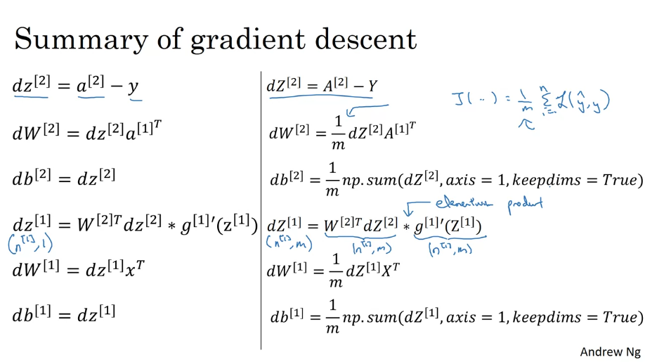
Random Initialization

Remember, $ W^{[1]} $ is the matrix of weights for layer 1, with dimensions:

Rows: number of activation units (ie nodes) in layer 1
Columns: number of input units (ie features for L1)

If weights are initialized to zero in a NN, then for any given example in the training set, $ a_1^{[1]} = a_2^{[1]} $. Hidden units like these have identical outputs and are called “symmetrical”. Then, for every step of Gradient Descent, every row of the dW matrix will be identical also.

In general, initializing all the weights to zero results in the network failing to break symmetry. This means that every neuron in each layer will learn the same thing, and you might as well be training a neural network with $ n^{[l]}=1 $ for every layer, and the network is no more powerful than a linear classifier such as logistic regression. Therefore, the goal is to have different activation functions in each hidden unit.

Note: initializing b^[1] to zero is not a problem.

Recommended approach:

W^[1] = np.random.randn((2,2)) * 0.01
b^[1] = np.zero((2,1))

The intuition behind the 0.01 constant multiplication in the initialization stage is to avoid large numbers in the calculation for $Z$. Large numbers move the value in the activatuion function towards the tails, which in turn makes the derivative fairly small, thus slowing down Gradient Descent, we want to avoid this.

Week 4

Deep Neural Net Notation

DNN notation

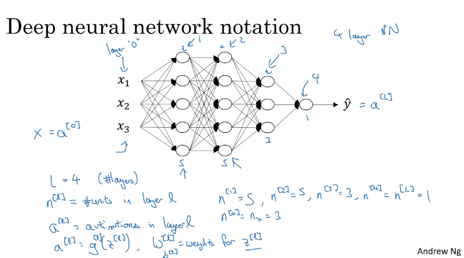
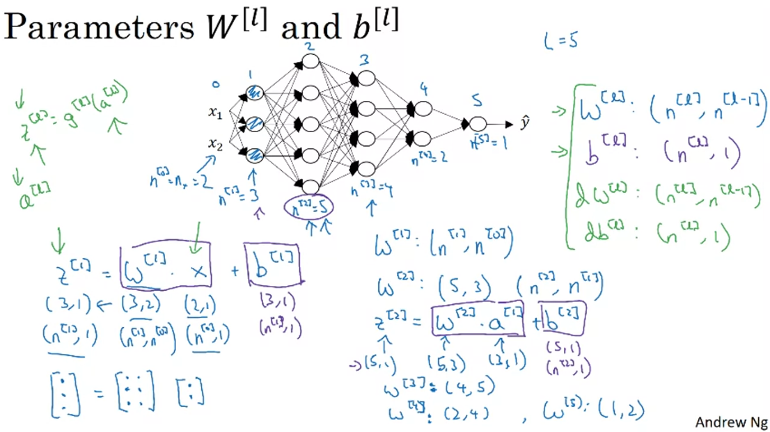
Dimensions for a single example

DNN dimensions

Forward and Backward Prop

DNN propagation

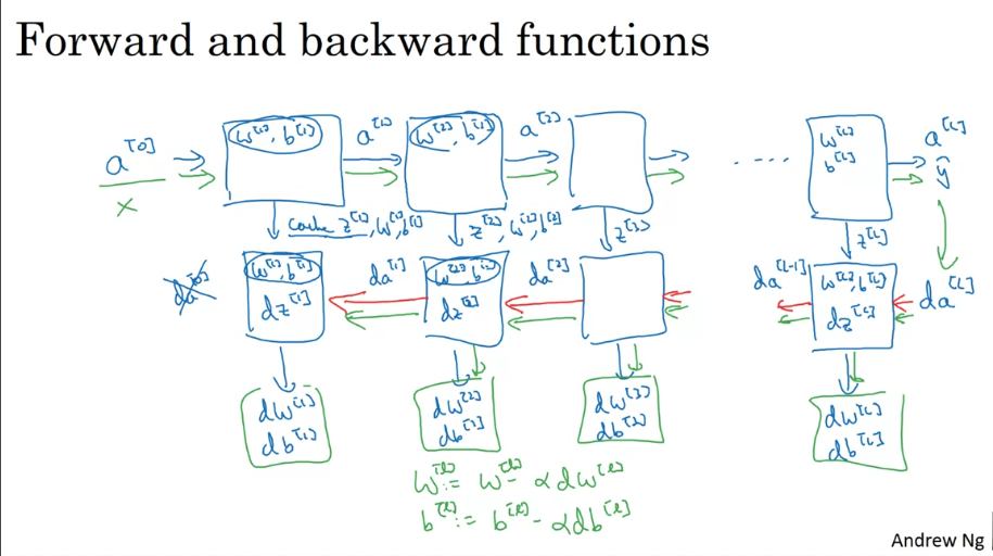
Forward Propagation

Vectorized version:
$ Z^{[l]}=W^{[l]}A^{[l-1]}+b^{[l]} $ (1)
$ A^{[l]}=g^{[l]}(Z^{[l]}) $ (2)

Note: the final activation function is the final output (ie prediction)
Note2: there is an unavoidable for loop to iterate through the layers

Backward Propagation

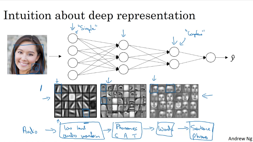
Deep NN Representation Depth